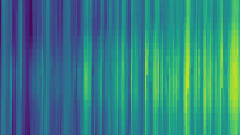
Visualization & Quality Analysis

This notebook demonstrates how to analyze the quality of time series aggregation using tsam’s built-in plotting tools.

We will:

1. Load and aggregate time series data

2. Visualize the original vs reconstructed data

3. Analyze cluster structure and assignments

4. Examine residuals and error patterns

5. Compare different aggregation configurations

6. Analyze segmentation results

import pandas as pd
import plotly.express as px
import plotly.io as pio

import tsam
from tsam import ClusterConfig, ExtremeConfig, SegmentConfig

pio.renderers.default = "notebook"

1. Load Data and Run Aggregation

# Load test data (8760 hours = 1 year of hourly data)
raw = pd.read_csv("testdata.csv", index_col=0)
print(f"Data shape: {raw.shape}")
print(f"Columns: {list(raw.columns)}")
raw.head()

Data shape: (8760, 4)
Columns: ['GHI', 'T', 'Wind', 'Load']

	GHI	T	Wind	Load
2009-12-31 23:30:00	0	-2.1	7.1	375.478394
2010-01-01 00:30:00	0	-2.8	8.6	364.541326
2010-01-01 01:30:00	0	-3.3	9.7	357.416844
2010-01-01 02:30:00	0	-3.2	9.8	350.191306
2010-01-01 03:30:00	0	-3.2	9.4	345.161449

# Run aggregation with 12 typical days
result = tsam.aggregate(
    raw,
    n_clusters=12,
    period_duration=24,
    cluster=ClusterConfig(method="hierarchical"),
)

print(f"Number of clusters: {result.n_clusters}")
print(f"Timesteps per period: {result.n_timesteps_per_period}")
print(f"Total original periods: {len(raw) // result.n_timesteps_per_period}")

Number of clusters: 12
Timesteps per period: 24
Total original periods: 365

2. Visual Comparison: Original vs Reconstructed

Heatmaps

Heatmaps show the full year with periods (days) on the x-axis and timesteps (hours) on the y-axis.

Use tsam.unstack_to_periods() to reshape data for heatmap visualization with plotly.

# Reshape raw data for heatmap visualization
unstacked = tsam.unstack_to_periods(raw, period_duration=24)

# Create heatmap with plotly express
px.imshow(
    unstacked["T"].values.T,
    labels={"x": "Day", "y": "Hour", "color": "Temperature"},
    title="Original Temperature",
    aspect="auto",
)

# Original data heatmap using result.original
unstacked_orig = tsam.unstack_to_periods(result.original, period_duration=24)
px.imshow(
    unstacked_orig["T"].values.T,
    labels={"x": "Day", "y": "Hour", "color": "Temperature"},
    title="Original Temperature (from result)",
    aspect="auto",
)

# Reconstructed data heatmap using result.reconstructed
unstacked_recon = tsam.unstack_to_periods(result.reconstructed, period_duration=24)
px.imshow(
    unstacked_recon["T"].values.T,
    labels={"x": "Day", "y": "Hour", "color": "Temperature"},
    title="Reconstructed Temperature",
    aspect="auto",
)

# Multi-column heatmaps of reconstructed data
for col in ["GHI", "T", "Load"]:
    px.imshow(
        unstacked_recon[col].values.T,
        labels={"x": "Day", "y": "Hour", "color": col},
        title=f"Reconstructed {col}",
        aspect="auto",
    ).show()

# Compare original vs reconstructed for specific columns
for col in ["T", "Load"]:
    fig_orig = px.imshow(
        unstacked_orig[col].values.T,
        labels={"x": "Day", "y": "Hour", "color": col},
        title=f"Original {col}",
        aspect="auto",
    )
    fig_orig.show()
    fig_recon = px.imshow(
        unstacked_recon[col].values.T,
        labels={"x": "Day", "y": "Hour", "color": col},
        title=f"Reconstructed {col}",
        aspect="auto",
    )
    fig_recon.show()

Duration Curves

Duration curves show sorted values and reveal how well the aggregation preserves the value distribution.

Use the result.plot.compare() accessor method for easy comparison.

# Duration curve with plotly express (raw data)
frames = []
for col in ["Load", "GHI"]:
    sorted_vals = raw[col].sort_values(ascending=False).reset_index(drop=True)
    frames.append(
        pd.DataFrame(
            {"Hour": range(len(sorted_vals)), "Value": sorted_vals, "Column": col}
        )
    )
long_df = pd.concat(frames, ignore_index=True)

px.line(long_df, x="Hour", y="Value", color="Column", title="Original Duration Curves")

# Accessor: Compare original vs reconstructed duration curves
result.plot.compare(mode="duration_curve")

# Duration curves for reconstructed data with plotly express
frames = []
for col in result.reconstructed.columns:
    sorted_vals = (
        result.reconstructed[col].sort_values(ascending=False).reset_index(drop=True)
    )
    frames.append(
        pd.DataFrame(
            {"Hour": range(len(sorted_vals)), "Value": sorted_vals, "Column": col}
        )
    )
long_df = pd.concat(frames, ignore_index=True)

px.line(
    long_df, x="Hour", y="Value", color="Column", title="Reconstructed Duration Curves"
)

Time Series Comparison

Compare original vs reconstructed as time series. Use plotly’s interactive zoom/pan to explore specific time periods.

# Accessor: Compare overlay mode (same color per column, dash differentiates Original/Reconstructed)
# Use plotly's interactive zoom to explore specific time ranges
result.plot.compare(
    columns=["T", "Load"],
    mode="overlay",
    title="Temperature and Load Comparison (use zoom to explore)",
)

# Accessor: Compare side-by-side mode
result.plot.compare(
    columns=["GHI"],
    mode="side_by_side",
    title="Solar Irradiance Comparison (side_by_side)",
)

3. Cluster Analysis

Understanding the cluster structure helps assess whether the aggregation captures meaningful patterns.

# Cluster weights - how many days are represented by each typical day
result.plot.cluster_weights()

# Cluster assignments - which cluster each original day belongs to
print("Cluster assignments (first 30 days):")
print(result.cluster_assignments[:30])
print(f"\nTotal periods: {len(result.cluster_assignments)}")

Cluster assignments (first 30 days):
[ 5 10  3  7  7  5  2  3  3  2  2  5  5  2  2  2  2  2  8  8  2  2  2  2
  2  5  8  2  2  2]

Total periods: 365

# Representative profiles for temperature
result.plot.cluster_representatives(columns=["T"])

# Representative profiles for solar irradiance
result.plot.cluster_representatives(columns=["GHI"])

4. Error Analysis

Accuracy Metrics

# Overall accuracy metrics
print("Accuracy Summary:")
print(result.accuracy)
print("\nRMSE per column:")
print(result.accuracy.rmse)
print("\nMAE per column:")
print(result.accuracy.mae)

Accuracy Summary:
AccuracyMetrics(
  rmse=0.0988 (mean),
  mae=0.0692 (mean),
  rmse_duration=0.0277 (mean)
)

RMSE per column:
GHI     0.086993
Load    0.085108
T       0.085319
Wind    0.137713
Name: RMSE, dtype: float64

MAE per column:
GHI     0.045101
Load    0.059208
T       0.066456
Wind    0.106038
Name: MAE, dtype: float64

# Visual comparison of accuracy metrics
result.plot.accuracy()

Residual Analysis

Residuals (original - reconstructed) reveal where the aggregation performs well or poorly.

# Residuals over time (mode="time_series")
result.plot.residuals(columns=["Load"], mode="time_series")

# Residual distribution (mode="histogram")
result.plot.residuals(columns=["T", "Load"], mode="histogram")

# Error by period (mode="by_period")
result.plot.residuals(columns=["Load"], mode="by_period")

# Error by timestep within period (mode="by_timestep")
result.plot.residuals(columns=["Load", "GHI"], mode="by_timestep")

5. Comparing Aggregation Configurations

Compare different numbers of clusters to see the accuracy-complexity tradeoff.

# Run aggregations with different cluster counts
results = {}
for n in [4, 8, 12, 24]:
    results[f"{n} clusters"] = tsam.aggregate(
        raw,
        n_clusters=n,
        period_duration=24,
        cluster=ClusterConfig(method="hierarchical"),
    )

# Print accuracy comparison
print("RMSE comparison (Load):")
for name, res in results.items():
    print(f"  {name}: {res.accuracy.rmse['Load']:.2f}")

# Build comparison data for plotting
comparison_data = {"Original": raw}
for name, res in results.items():
    comparison_data[name] = res.reconstructed

RMSE comparison (Load):
  4 clusters: 0.14
  8 clusters: 0.10
  12 clusters: 0.09
  24 clusters: 0.07

# Compare duration curves across configurations with plotly express
frames = []
for name, df in comparison_data.items():
    sorted_vals = df["Load"].sort_values(ascending=False).reset_index(drop=True)
    frames.append(
        pd.DataFrame(
            {"Hour": range(len(sorted_vals)), "Load": sorted_vals, "Method": name}
        )
    )
long_df = pd.concat(frames, ignore_index=True)

px.line(
    long_df,
    x="Hour",
    y="Load",
    color="Method",
    title="Duration Curve: Cluster Count Comparison",
)

# Time slice comparison with plotly express
frames = []
for name, df in comparison_data.items():
    sliced = df.loc["20100601":"20100608", ["Load"]].copy()
    sliced["Method"] = name
    frames.append(sliced)
long_df = pd.concat(frames).reset_index(names="Time")

px.line(
    long_df,
    x="Time",
    y="Load",
    color="Method",
    title="June Week: Cluster Count Comparison",
)

6. Effect of Extreme Period Preservation

Compare aggregation with and without preserving extreme values.

# Without extreme preservation
result_no_extremes = tsam.aggregate(
    raw,
    n_clusters=8,
    period_duration=24,
    cluster=ClusterConfig(method="hierarchical"),
)

# With extreme preservation
result_with_extremes = tsam.aggregate(
    raw,
    n_clusters=8,
    period_duration=24,
    cluster=ClusterConfig(method="hierarchical"),
    extremes=ExtremeConfig(
        method="new_cluster",
        min_value=["T"],
        max_value=["Load", "GHI"],
    ),
)

print("Without extremes - Load RMSE:", result_no_extremes.accuracy.rmse["Load"])
print("With extremes - Load RMSE:", result_with_extremes.accuracy.rmse["Load"])

Without extremes - Load RMSE: 0.10117201266675802
With extremes - Load RMSE: 0.09728116855411595

# Compare peak preservation in duration curves with plotly express
comparison_extremes = {
    "Original": raw,
    "No extremes": result_no_extremes.reconstructed,
    "With extremes": result_with_extremes.reconstructed,
}

frames = []
for name, df in comparison_extremes.items():
    sorted_vals = df["Load"].sort_values(ascending=False).reset_index(drop=True)
    frames.append(
        pd.DataFrame(
            {"Hour": range(len(sorted_vals)), "Load": sorted_vals, "Method": name}
        )
    )
long_df = pd.concat(frames, ignore_index=True)

px.line(
    long_df,
    x="Hour",
    y="Load",
    color="Method",
    title="Effect of Extreme Period Preservation on Load",
)

# Compare temperature extremes with plotly express
frames = []
for name, df in comparison_extremes.items():
    sorted_vals = df["T"].sort_values(ascending=False).reset_index(drop=True)
    frames.append(
        pd.DataFrame(
            {
                "Hour": range(len(sorted_vals)),
                "Temperature": sorted_vals,
                "Method": name,
            }
        )
    )
long_df = pd.concat(frames, ignore_index=True)

px.line(
    long_df,
    x="Hour",
    y="Temperature",
    color="Method",
    title="Effect of Extreme Period Preservation on Temperature",
)

7. Segmentation Analysis

When using segmentation, you can visualize the segment durations.

# Run aggregation with segmentation
result_segmented = tsam.aggregate(
    raw,
    n_clusters=12,
    period_duration=24,
    cluster=ClusterConfig(method="hierarchical"),
    segments=SegmentConfig(n_segments=6),
)

print(f"Segments per period: {len(result_segmented.segment_durations[0])}")
print(f"Segment durations (first cluster): {result_segmented.segment_durations[0]}")

Segments per period: 6
Segment durations (first cluster): (7, 2, 5, 3, 5, 2)

# Plot segment durations
result_segmented.plot.segment_durations()

# Compare segmented vs non-segmented with plotly express
comparison_seg = {
    "Original": raw,
    "No segmentation": result.reconstructed,
    "With segmentation": result_segmented.reconstructed,
}

frames = []
for name, df in comparison_seg.items():
    sorted_vals = df["Load"].sort_values(ascending=False).reset_index(drop=True)
    frames.append(
        pd.DataFrame(
            {"Hour": range(len(sorted_vals)), "Load": sorted_vals, "Method": name}
        )
    )
long_df = pd.concat(frames, ignore_index=True)

px.line(
    long_df,
    x="Hour",
    y="Load",
    color="Method",
    title="Effect of Segmentation on Load Duration Curve",
)

Summary

Plotting Overview

For heatmaps - use ``tsam.unstack_to_periods()`` with plotly:

import plotly.express as px
unstacked = tsam.unstack_to_periods(df, period_duration=24)
px.imshow(unstacked["Load"].values.T, labels={"x": "Day", "y": "Hour", "color": "Load"})

Accessor methods (``result.plot.*``) - for validation after aggregation:

• compare(columns, mode) - Compare original vs reconstructed

  • mode="overlay" - Same plot, color=column, dash=source

  • mode="side_by_side" - Faceted by source

  • mode="duration_curve" - Sorted value comparison

  • Use plotly’s interactive zoom/pan to explore specific time ranges

• residuals(columns, mode) - Error analysis

  • mode="time_series" - Residuals over time

  • mode="histogram" - Error distribution

  • mode="by_period" - MAE per original period

  • mode="by_timestep" - MAE by hour within period

• cluster_weights() - Bar chart of cluster sizes

• cluster_representatives(columns) - Line plots of typical periods

• accuracy() - Bar chart of RMSE/MAE metrics

• segment_durations() - Bar chart of segment lengths (requires segmentation)

Data properties (``result.*``) - for direct access:

• result.original - Original DataFrame

• result.reconstructed - Reconstructed DataFrame (cached)

• result.residuals - Difference: original - reconstructed

• result.cluster_assignments - Array of cluster indices per period